Hands-on Exercise 5: Ternary Plot

1. Plotting Ternary Diagram with R

Install and launching R packages.

The code chunk below uses p_load() of pacman package to check if packages are installed in the computer. If they are, then they will be launched into R. The R packages installed are:

• ggtern, a ggplot extension specially designed to plot ternary diagrams. The package will be used to plot static ternary plots.
• Plotly R, an R package for creating interactive web-based graphs via plotly’s JavaScript graphing library, plotly.js . The plotly R libary contains the ggplotly function, which will convert ggplot2 figures into a Plotly object.

pacman::p_load(ggtern, plotly, tidyverse)

Importing the data

pop_data <- read_csv("data/respopagsex2000to2018_tidy.csv") 

Preparing the data

agpop_mutated <- pop_data %>%
  mutate(`Year` = as.character(Year))%>%
  spread(AG, Population) %>%
  mutate(YOUNG = rowSums(.[4:8]))%>%
  mutate(ACTIVE = rowSums(.[9:16]))  %>%
  mutate(OLD = rowSums(.[17:21])) %>%
  mutate(TOTAL = rowSums(.[22:24])) %>%
  filter(Year == 2018)%>%
  filter(TOTAL > 0)

agpop_mutated

# A tibble: 234 × 25
   PA        SZ    Year  AGE0-…¹ AGE05…² AGE10…³ AGE15…⁴ AGE20…⁵ AGE25…⁶ AGE30…⁷
   <chr>     <chr> <chr>   <dbl>   <dbl>   <dbl>   <dbl>   <dbl>   <dbl>   <dbl>
 1 Ang Mo K… Ang … 2018      180     270     320     300     260     300     270
 2 Ang Mo K… Chen… 2018     1060    1080    1080    1260    1400    1880    1940
 3 Ang Mo K… Chon… 2018      900     900    1030    1220    1380    1760    1830
 4 Ang Mo K… Kebu… 2018      720     850    1010    1120    1230    1460    1330
 5 Ang Mo K… Semb… 2018      220     310     380     500     550     500     300
 6 Ang Mo K… Shan… 2018      550     630     670     780     950    1080     990
 7 Ang Mo K… Tago… 2018      260     340     430     500     640     690     440
 8 Ang Mo K… Town… 2018      830     930     930     860    1020    1400    1350
 9 Ang Mo K… Yio … 2018      160     160     220     260     350     340     230
10 Ang Mo K… Yio … 2018      810    1070    1300    1450    1500    1590    1390
# … with 224 more rows, 15 more variables: `AGE35-39` <dbl>, `AGE40-44` <dbl>,
#   `AGE45-49` <dbl>, `AGE50-54` <dbl>, `AGE55-59` <dbl>, `AGE60-64` <dbl>,
#   `AGE65-69` <dbl>, `AGE70-74` <dbl>, `AGE75-79` <dbl>, `AGE80-84` <dbl>,
#   AGE85over <dbl>, YOUNG <dbl>, ACTIVE <dbl>, OLD <dbl>, TOTAL <dbl>, and
#   abbreviated variable names ¹​`AGE0-4`, ²​`AGE05-9`, ³​`AGE10-14`, ⁴​`AGE15-19`,
#   ⁵​`AGE20-24`, ⁶​`AGE25-29`, ⁷​`AGE30-34`

Static Ternary Diagram

ggtern(data = agpop_mutated,
       aes(x = YOUNG,
           y = ACTIVE,
           z = OLD)) +
  geom_point() +
  labs(title = "Population structure, 2015") +
  theme_rgbw()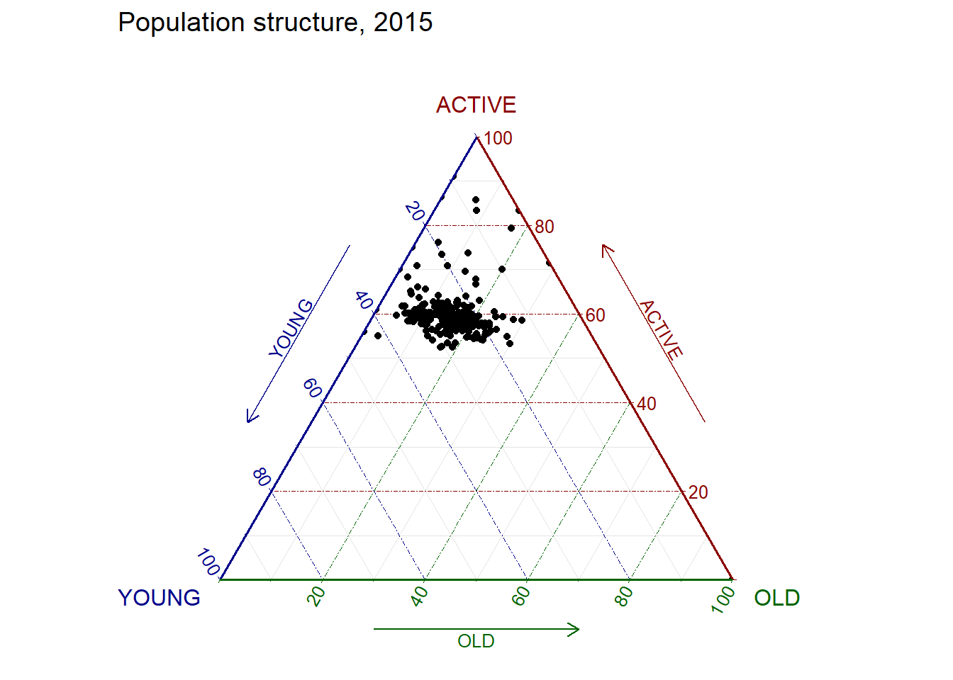

Interactive Ternary Diagram

label <- function(txt) {
  list(
    text = txt, 
    x = 0.1, y = 1,
    ax = 0, ay = 0,
    xref = "paper", yref = "paper", 
    align = "center",
    font = list(family = "serif", size = 15, color = "white"),
    bgcolor = "#b3b3b3", bordercolor = "black", borderwidth = 2
  )
}

axis <- function(txt) {
  list(
    title = txt, tickformat = ".0%", tickfont = list(size = 10)
  )
}

ternaryAxes <- list(
  aaxis = axis("Young"), 
  baxis = axis("Active"), 
  caxis = axis("Old")
)

plot_ly(
  data = agpop_mutated, 
  a = ~YOUNG, 
  b = ~ACTIVE, 
  c = ~OLD, 
  color = I("black"), 
  type = "scatterternary"
) |> 
  layout(
    annotations = label("Ternary Markers"), 
    ternary = ternaryAxes
  )