In-class Exercise 4

1. Install and loading R packages

Packages will be installed and loaded. Note that performance, parameters, see are under easystats

pacman::p_load(plotly, DT, patchwork, ggstatsplot, readxl, performance, parameters, see, gtsummary, tidyverse)

2. Importing Data

exam_data <- read_csv("data/Exam_data.csv")

car_resale <- read_xls("data/ToyotaCorolla.xls", 
                       "data")

3. Interactivity in plotting

Plotting with native plot_ly()

plot_ly(data = exam_data,
        x = ~ENGLISH,
        y = ~MATHS,
        color = ~RACE)

Plotting with ggplot2 and wrapped with ggplotly()

Note that only native ggplot2 can be used

p <- ggplot(data=exam_data, 
            aes(x = MATHS,
                y = ENGLISH,
                color = RACE)) +
  geom_point(size = 1) +
  coord_cartesian(xlim=c(0,100),
                  ylim=c(0,100))
ggplotly(p) 

4. Visual statistical plotting

Two-sample mean testing

ggbetweenstats(
  data = exam_data,
  x = GENDER,
  y = MATHS,
  #"p" is parametric test while "np" is non-parametric test
  type = "p",
  messages = FALSE
)

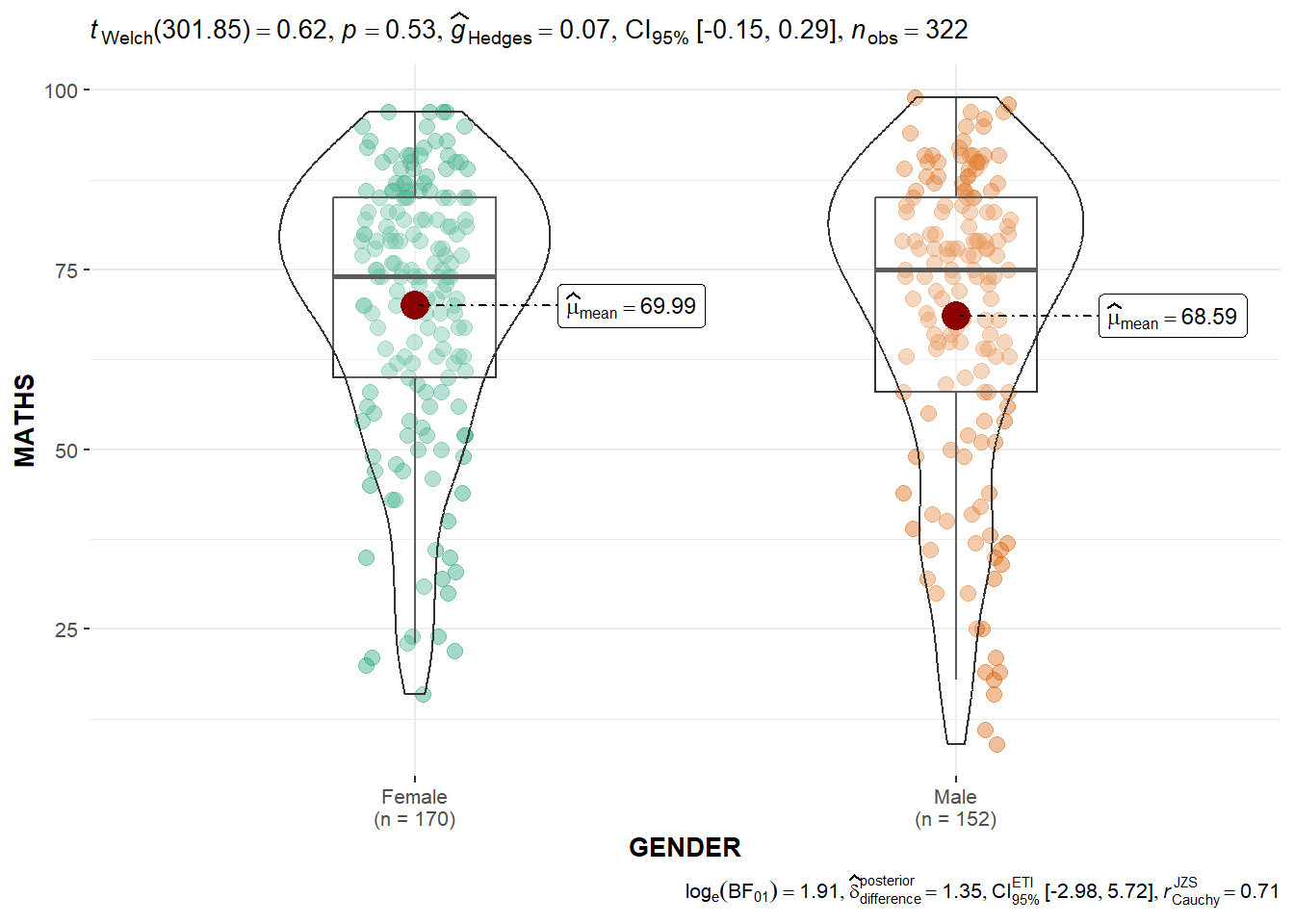
Bayesian test (bottom-right) is only displayed for parametric test (normality assumption) as they are comparing the mean. Note that Welch test is used as it does not assume equal variance.

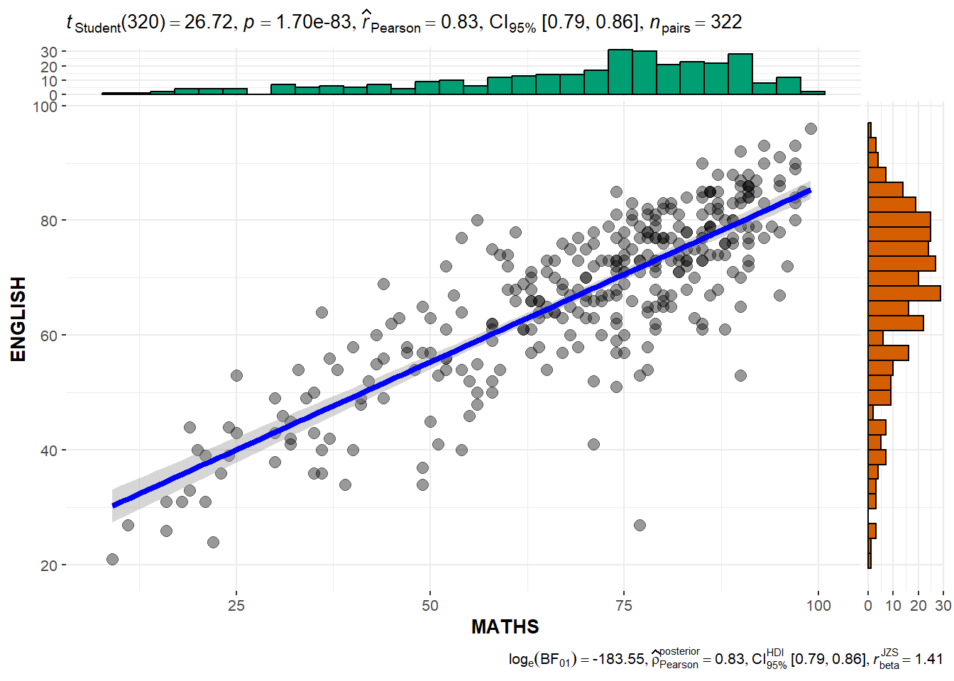
Scatterplot testing

ggscatterstats(
  data = exam_data,
  x = MATHS,
  y = ENGLISH,
  #the default for marginal is TRUE which will show the marginal plots
  marginal = TRUE
)

5. Model visualization

Building least-square multiple regression model

lm() is base R model to build least-square multiple regression model

model <- lm(Price ~ Age_08_04 + Mfg_Year + KM +
              Weight + Guarantee_Period, data = car_resale)
model

Call:
lm(formula = Price ~ Age_08_04 + Mfg_Year + KM + Weight + Guarantee_Period, 
    data = car_resale)

Coefficients:
     (Intercept)         Age_08_04          Mfg_Year                KM  
      -2.637e+06        -1.409e+01         1.315e+03        -2.323e-02  
          Weight  Guarantee_Period  
       1.903e+01         2.770e+01  

Use gtsummary to summarize data sets, regression models, and more, using sensible defaults with highly customisable capabilities.

Diagnostic test : Check for multi-collinearity

Visualizing multi-collinearity of the model.

Note that check_c is a dataframe.

check_c <- check_collinearity(model)
plot(check_c)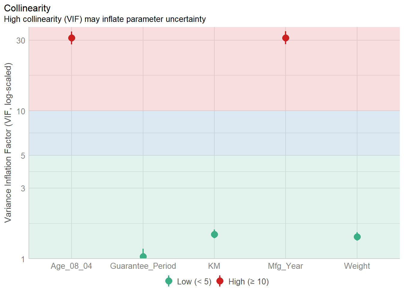

Diagnostic test : Check for normality assumption

#Remove Mfg_Year from model due to high collinearity
model1 <- lm(Price ~ Age_08_04 + KM + 
              Weight + Guarantee_Period, data = car_resale)
model1

Call:
lm(formula = Price ~ Age_08_04 + KM + Weight + Guarantee_Period, 
    data = car_resale)

Coefficients:
     (Intercept)         Age_08_04                KM            Weight  
      -2.186e+03        -1.195e+02        -2.406e-02         1.972e+01  
Guarantee_Period  
       2.682e+01  

Visualizing normality assumption of the model.

Note that check_n is a dataframe.

check_n <- check_normality(model1)
plot(check_n)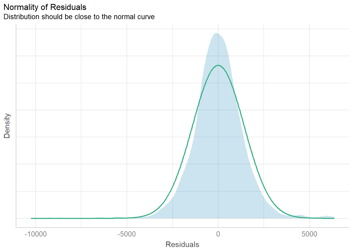

Diagnostic test : Check for variance homogeneity

Note that check_h is a dataframe.

check_h <- check_heteroscedasticity(model1)
plot(check_h)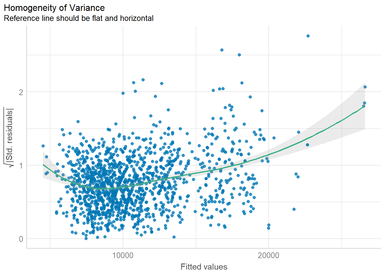

Diagnostic test : Check for everything

check_model(model1)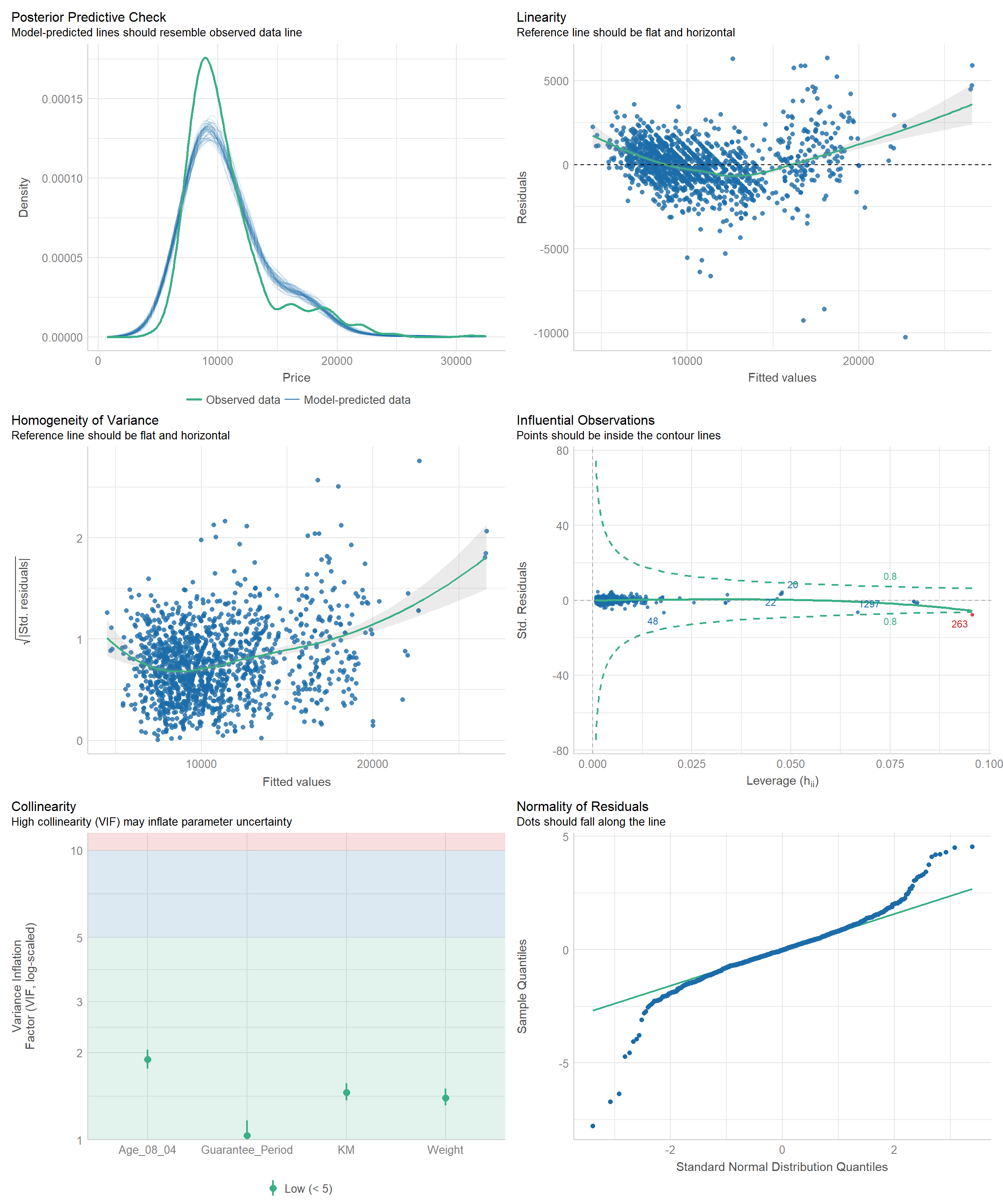

Visualizing regression parameters

plot(parameters(model1))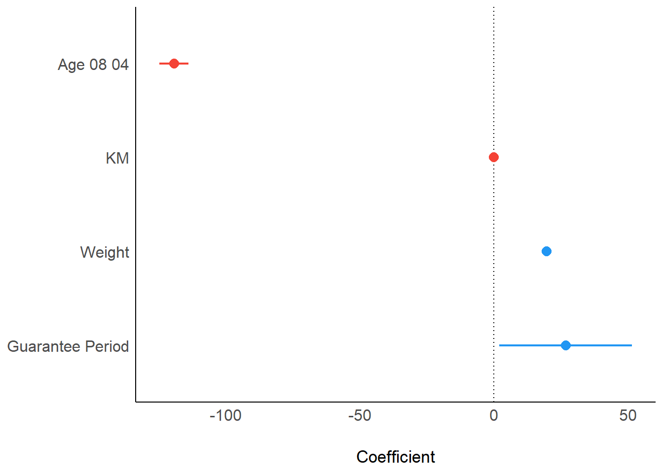

ggcoefstats(model1, 
            output = "plot")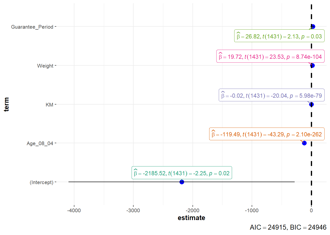

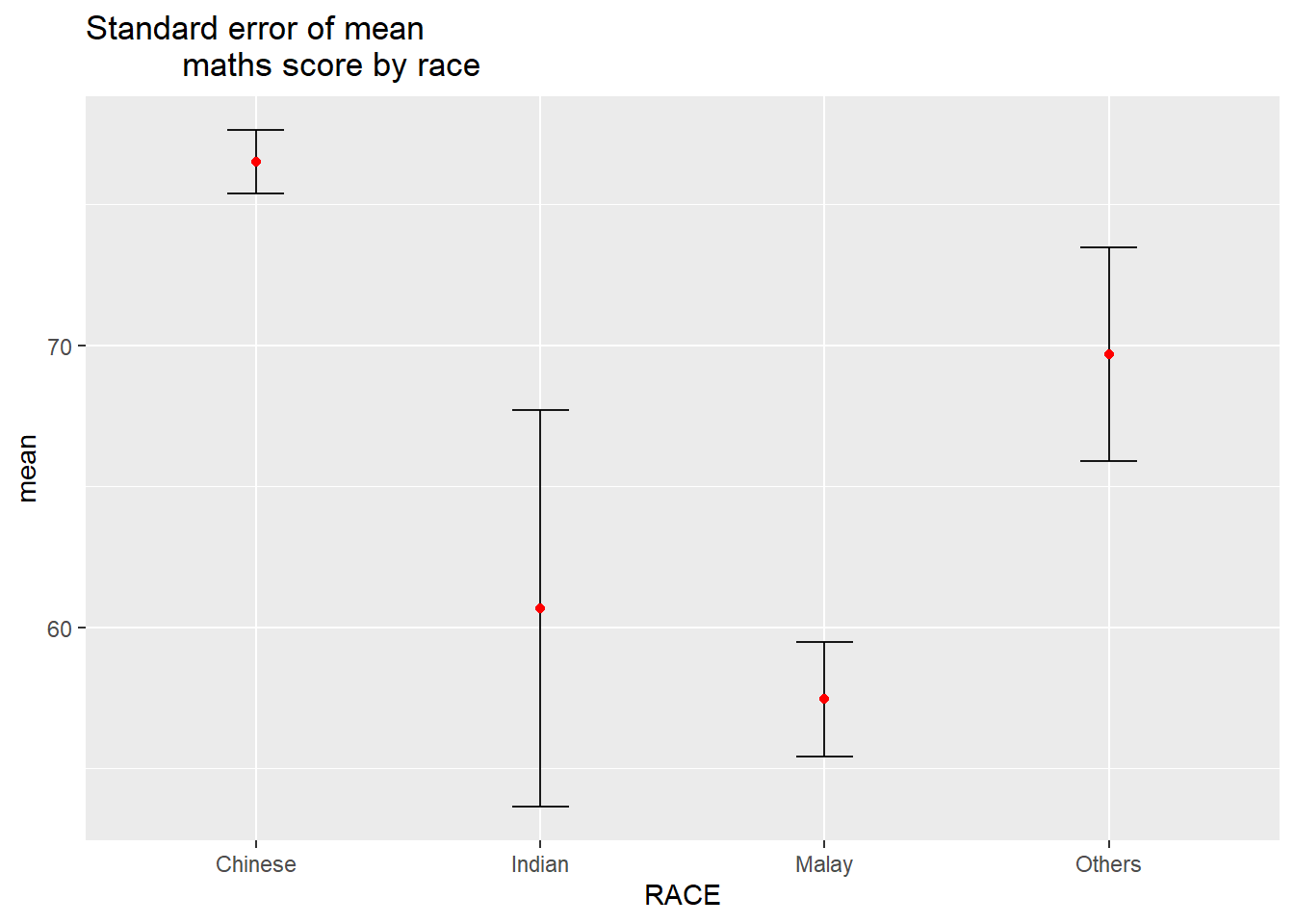
6. Visualization of uncertainty

Data preparation

#group by RACE and calculate mean, sd, and se of MATHS score
my_sum <- exam_data |> 
  group_by(RACE) |> 
  summarize(
    n = n(),
    mean = mean(MATHS),
    sd = sd(MATHS)) |>
  mutate(se = sd/sqrt(n-1))

Plotting using ggplot2

ggplot(my_sum) +
  
  geom_errorbar(
    aes(x = RACE,
        ymin = mean - se,
        ymax = mean + se),
    width = 0.2,
    colour = "black",
    alpha = 0.9,
    linewidth = 0.5) +
  
  geom_point(
    aes(x = RACE,
        y = mean),
    stat = "identity",
    colour = "red",
    size = 1.5,
    alpha = 1) +
  
  ggtitle("Standard error of mean
          maths score by race")